Mapping Twitter Followers in R
05 Apr 2016
My colleague Jon Lieber and I recently released a new report that analyzes how digital marketplaces that connect workers to consumers demanding their services (e.g. Uber, Thumbtack, Upwork, etc.) are affecting the American labor market. As part of this report, we looked at where these digital marketplaces are most active. Although the biggest ones are now active throughout the United States, their dispersion patterns are far from uniform. How did we find this out? Well, we started by turning to readily accessible data source: Twitter, with the theory that platforms with more Twitter followers in a given area will also be more active in that area.
 Using Geoff Jentry’s
 twitteR package, we downloaded data on every follower that each of the 10 of the biggest digital marketplaces had at the time. We then geocoded these users’ locations (as self-reported in their bios) using the Google Maps API, doing so via a modified version of the geocode function in David Kahle and Hadley Wickham’s ggmap package. With this information, we then generated maps of each platform’s dispersion and measured their activity levels in markets across the country. While this approach isn’t perfect, it turns out to be pretty good. We know this because we compared Thumbtack’s Twitter follower locations to our internal marketplace data and the two are strongly correlated (for a similar use of Twitter data to generate spatial insights, see Simon Rogers’ NFL fan map).
This post will show you to reproduce this methodology for your own purposes using a simple example: mapping my own Twitter followers.
Step 1: Enable Pings to the Twitter API
To access the Twitter API, the first thing you’ll need to do is register with them via apps.twitter.com. Once you do so, you’ll be given the following: Consumer Key (API Key), Consumer Secret (API Secret), Access Token, and an Access Token Secret. You can then move into R. There, you’ll want to install and load the twitteR package and then use the package to establish your API credentials:
if (!require("twitteR")) {
  install.packages("twitteR", repos="http://cran.rstudio.com/")
  library("twitteR")
}
consumer_key <- "[YOUR CONSUMER KEY HERE]"
consumer_secret <- "[YOUR CONSUMER SECRET HERE]"
access_token <- "[YOUR ACCESS TOKEN HERE]"
access_secret <- "[YOUR ACCESS SECRET HERE]"
options(httr_oauth_cache=T) #This will enable the use of a local file to cache OAuth access credentials between R sessions.
setup_twitter_oauth(consumer_key,
                    consumer_secret,
                    access_token,
                    access_secret)
After running this code, you should see the following:
## [1] "Using direct authentication"
Step 2: Download the Followers of a Given Twitter Account
You’re now ready to ping the Twitter account; fortunately, the twitteR package makes this fairly easy. As a first step, you can download info on a given user and take a look their location, as they report in their Twitter bio:
lucaspuente <- getUser("lucaspuente")
location(lucaspuente)
## [1] "SF"
You can then move onto to downloading data on this user’s followers. You can obtain this information by simply running the getFollowers() function.
In this particular example, I don’t have too many followers (333 at the time of writing), so I don’t have to worry about exceeding the API’s limits when making a call to download data on all of my followers at once. This will be a concern, though, if you’re interested in downloading data on the followers of an account that has more than a few thousand. In that case, you’ll want tell R to retry the Twitter API after it’s been “rate limited”. You can do so by including the optional retryOnRateLimit argument to ensure that you end up downloading data on the account’s full set of followers and don’t get cut off by the Twitter API before then.
lucaspuente_follower_IDs<-lucaspuente$getFollowers(retryOnRateLimit=180)
You can double check that you successfully pulled data on every follower of the account by ensuring that the length of this new list you just generated is the same as the number of followers you know that the account has.
length(lucaspuente_follower_IDs)
## [1] 333
Since we see we’re good here, we can move on.
Step 3: Organize the Data You’ve Just Acquired
The next step is turn this list of Twitter followers into a data frame. You don’t necessarily have to do this, but I generally find it more intuitive to deal with data frames than lists. If you do proceed with this step, I recommend using this combination of lapply() and rbindlist() (from the data.table package). Though there are a bunch of other ways to do this, I found this one to be a nice mix of code parsimony and processing speed.
if (!require("data.table")) {
  install.packages("data.table", repos="http://cran.rstudio.com/")
  library("data.table")
}
lucaspuente_followers_df = rbindlist(lapply(lucaspuente_follower_IDs,as.data.frame))
Once you’ve done this, I recommend taking a quick look at the types of data you’ll be dealing with when thinking about the locations of the Twitter account’s followers.
head(lucaspuente_followers_df$location, 10)
##  [1] "Lima, Peru"               "Israel"
##  [3] "Kingsport, Massachusetts" "San Diego, CA"
##  [5] "Wyoming, USA"             "Oakland, CA"
##  [7] ""                         "San Francisco"
##  [9] "Cambridge, MA"            ""
In this example, you immediately notice two things: 1) there are going to be decent number of followers that don’t list a location in their Twitter bio (these show up as "") and 2) what some users list as a location isn’t actually a location (e.g. ACA Forward #HeatNation). Dealing with the blanks is pretty easy: simply remove them from your data frame. We’ll deal with the second problem in the next step.
lucaspuente_followers_df<-subset(lucaspuente_followers_df, location!="")
Step 4: Geocode Followers’ Locations
Now you have the self-reported locations of the account’s Twitter followers, but you can’t yet map them since we don’t have any supplementary data to tell R where / how to plot an entry like SF (the location I report in my Twitter bio). To fix this, you’ll have to geocode them, but this isn’t too difficult thanks in part to David Kahle and Hadley Wickham’s ggmap package. It includes the very handy geocode() function that allows you to access the Google Maps API without having to leave R. You’re now almost ready to start using this function to ping the Google Maps API and geocode these locations, but before you can do that, you’ll need to do remove any instances of % since that character doesn’t play well with the API.
lucaspuente_followers_df$location<-gsub("%", " ",lucaspuente_followers_df$location)
Before you start, I also recommend creating an account in the Google Developers Console. Once you do so, you’ll be able to acquire an API key via the “Credentials” page in the Developers Console. This is a helpful step because, without registering (and agreeing to pay a very nominal amount per request), you can only use this API 2,500 times per day.
While the off-the-shelf geocode() function doesn’t allow you to enter your personalized key even if you have registered, you can can overcome this by using a modified version of the existing geocode() function so that calls to the Google Maps API are associated with your account. To help you with this, I’ve modified the raw code behind the geocode() function and edited line 174 so it reads like this:
  if(source == "google"){
    url_string <- paste("https://maps.googleapis.com/maps/api/geocode/json?address=", posturl, "&key=", api_key, sep = "")
  }...
You can download and run this code via Github:
#Install key package helpers:
source("https://raw.githubusercontent.com/LucasPuente/geocoding/master/geocode_helpers.R")
#Install modified version of the geocode function
#(that now includes the api_key parameter):
source("https://raw.githubusercontent.com/LucasPuente/geocoding/master/modified_geocode.R")
Before you proceed with geocoding the location strings you acquired in Step 2, you’ll also need to generate a function that specifics exactly what you want to extract from the Google Maps API.
geocode_apply<-function(x){
    geocode(x, source = "google", output = "all", api_key="[INSERT YOUR GOOGLE API KEY HERE]")
}
This will allow you to execute this function over the entire vector of location strings (e.g. lucaspuente_followers_df$location) without having to rely on a for loop. Instead, you can use the more efficient sapply() function.
geocode_results<-sapply(lucaspuente_followers_df$location, geocode_apply, simplify = F)
This will return a list that’s as long as the number of locations that were geocoded; in this case that’s 244 out of 333 total followers (~74%).
length(geocode_results)
## [1] 245
Step 5: Clean Geocoding Results
I also mentioned above that some users will put information in the “location” section of their Twitter bio that really isn’t a location. Fortunately, the Google Maps API offers some help in dealing with those. For starters, the API will tell us if the location entered “was successfully parsed and at least one geocode was returned” by indicating that the “status” field within the geocoding response object is "ok". So, you’ll need to remove any locations that have a status that isn’t “ok”.
condition_a <- sapply(geocode_results, function(x) x["status"]=="OK")
geocode_results<-geocode_results[condition_a]
Also, if a location is particularly ambiguous, the Google Maps API will return any matching result. Since you don’t know which one of these (if any) is the one the user’s actual location, you’ll want to eliminate locations that don’t have exactly one match. Together, these two steps remove 43 entries or ~13% of the locations that were geocoded.
condition_b <- lapply(geocode_results, lapply, length)
condition_b2<-sapply(condition_b, function(x) x["results"]=="1")
geocode_results<-geocode_results[condition_b2]
length(geocode_results)
## [1] 202
One other check you’ll have to do is to look for misformatted entries (a potential issue when simultaneously dealing with addresses from across the world) and fix them when found. To help keep things clean, I posted a cleaning script on Github that you can just run yourself.
source("https://raw.githubusercontent.com/LucasPuente/geocoding/master/cleaning_geocoded_results.R")
Now that you’ve filtered out imprecise and misformatted results, you’re ready to turn this list into a data frame.
results_b<-lapply(geocode_results, as.data.frame)
Then, to simplify things, you should extract out only the columns you need to generate a map of this data.
results_c<-lapply(results_b,function(x) subset(x, select=c("results.formatted_address",
                                                           "results.geometry.location")))
However, since the longitude and latitude data are contained in two different rows in the results.geometry.location column, you’ll need to slightly reshape the data frames you’ve just created to turn these two rows into one.
results_d<-lapply(results_c,function(x) data.frame(Location=x[1,"results.formatted_address"],
                                                   lat=x[1,"results.geometry.location"],
                                                   lng=x[2,"results.geometry.location"]))
Now you have each individual data frame formatted properly, so you can go ahead and bind them together using the efficient rbindlist from the data.table package.
results_e<-rbindlist(results_d)
You can also add in a column to document the user-specified location strings that were successfully geocoded.
results_f<-results_e[,Original_Location:=names(results_d)]
Since the maps we’re ultimately interested in generating will show the spatial distribution of Twitter followers in the US, you should eliminate followers that are outside the country.
american_results<-subset(results_f,
                  grepl(", USA", results_f$Location)==TRUE)
Let’s quickly check how successful our geocoding and filtering has been so far.
head(american_results,5)
##                  Location      lat        lng        Original_Location
## 1:     Massachusetts, USA 42.40721  -71.38244 Kingsport, Massachusetts
## 2:     San Diego, CA, USA 32.71574 -117.16108            San Diego, CA
## 3:       Oakland, CA, USA 37.80436 -122.27111              Oakland, CA
## 4: San Francisco, CA, USA 37.77493 -122.41942            San Francisco
## 5:     Cambridge, MA, USA 42.37362  -71.10973            Cambridge, MA
You can see that Google has been fairly successfully in geocoding potentially ambiguous location strings. For example The Golden State turned into California, USA, which has its own coordinates. While this is generally helpful, such vague locations shouldn’t be mapped. That’s because you don’t know where in this big state the user is actually located and the coordinates of 36.77826, -119.41793 will place the person roughly in the middle of California, which is unlikely to be where they actually are.
You can deal with this, though, since any location that includes a city has two commas, while a location with just one comma only includes a state and is therefore too vague to be properly mapped. Our strategy is simply to eliminate any entries that don’t have exactly two commas.
american_results$commas<-sapply(american_results$Location, function(x)
  length(as.numeric(gregexpr(",", as.character(x))[[1]])))
american_results<-subset(american_results, commas==2)
#Drop the "commas" column:
american_results<-subset(american_results, select=-commas)
Now you’re done cleaning the results from the geocoding process and you can see that you’ve acquired “mappable” locations in the United States for 150 the 245 Twitter followers with non-blank locations, a success rate of 61%.
nrow(american_results)
## [1] 150
Step 6: Map the Geocoded Results
Now your data is ready to be mapped, but before you do so, you’ll need to install a few packages. To do so efficiently, I recommend using this handy function that can help you install and / or load multiple packages at once.
ipak <- function(pkg){
    new.pkg <- pkg[!(pkg %in% installed.packages()[, "Package"])]
    if (length(new.pkg))
        install.packages(new.pkg, dependencies = TRUE, repos="http://cran.rstudio.com/")
    sapply(pkg, require, character.only = TRUE)
}
packages <- c("maps", "mapproj")
ipak(packages)
The maps package is helpful because it comes with some ready-to-plot maps. With the below code, you’ll load a map of the United States with an Albers projection. When using this particular projection, you’ll need to specify the parameters: param=c(39, 45). For the coloring, we’re setting the lines of the map to grey (col="#999999") to make it easier to see what we really care about: the location of my Twitter followers.
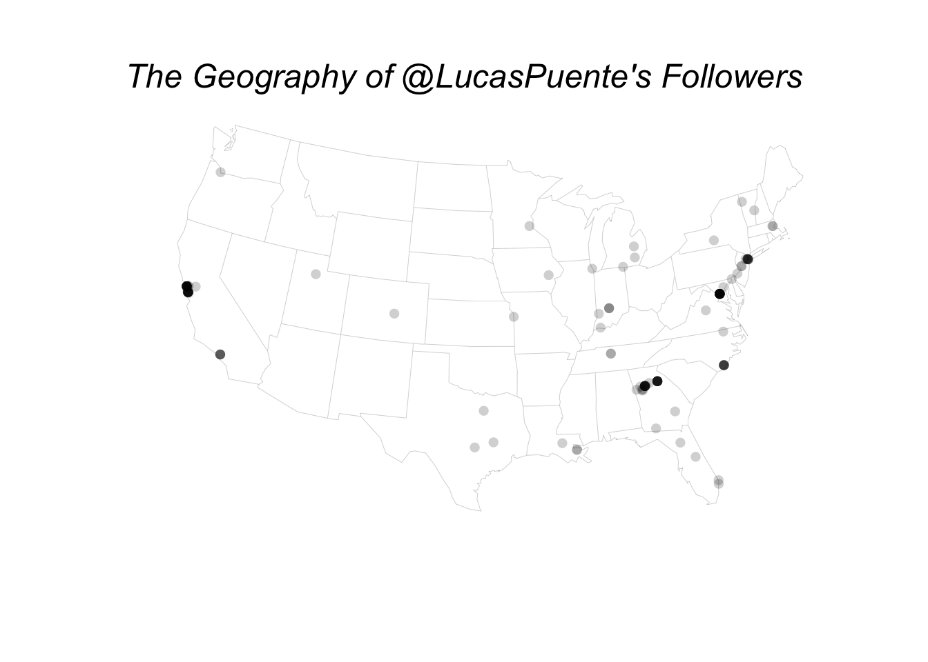
Now that you’ve created a map with only the outlines of the states, you’re ready to add the data. Since you’re using an Albers projection of the map, you’ll have to apply the same projection to the points, even though you already have each follower’s longitude and latitude. To do this, you’ll simply need to use the mapproject() function from the mapproj package. Add a title and your plot of the geography of @lucaspuente’s Twitter followers is complete!
#Generate a blank map:
albers_proj<-map("state", proj="albers", param=c(39, 45),
                 col="#999999", fill=FALSE, bg=NA, lwd=0.2, add=FALSE, resolution=1)
#Add points to it:
points(mapproject(american_results$lng, american_results$lat), col=NA, bg="#00000030", pch=21, cex=1.0)
#Add a title:
mtext("The Geography of @LucasPuente's Followers", side = 3, line = -3.5, outer = T, cex=1.5, font=3)
Inspired by Nathan Yau’s coffee shop maps, I followed his lead in turning this into a smoothed density map. The results are presented below, though you should sign up for a membership on his site if you want to see the exact code you’ll need to recreate it.
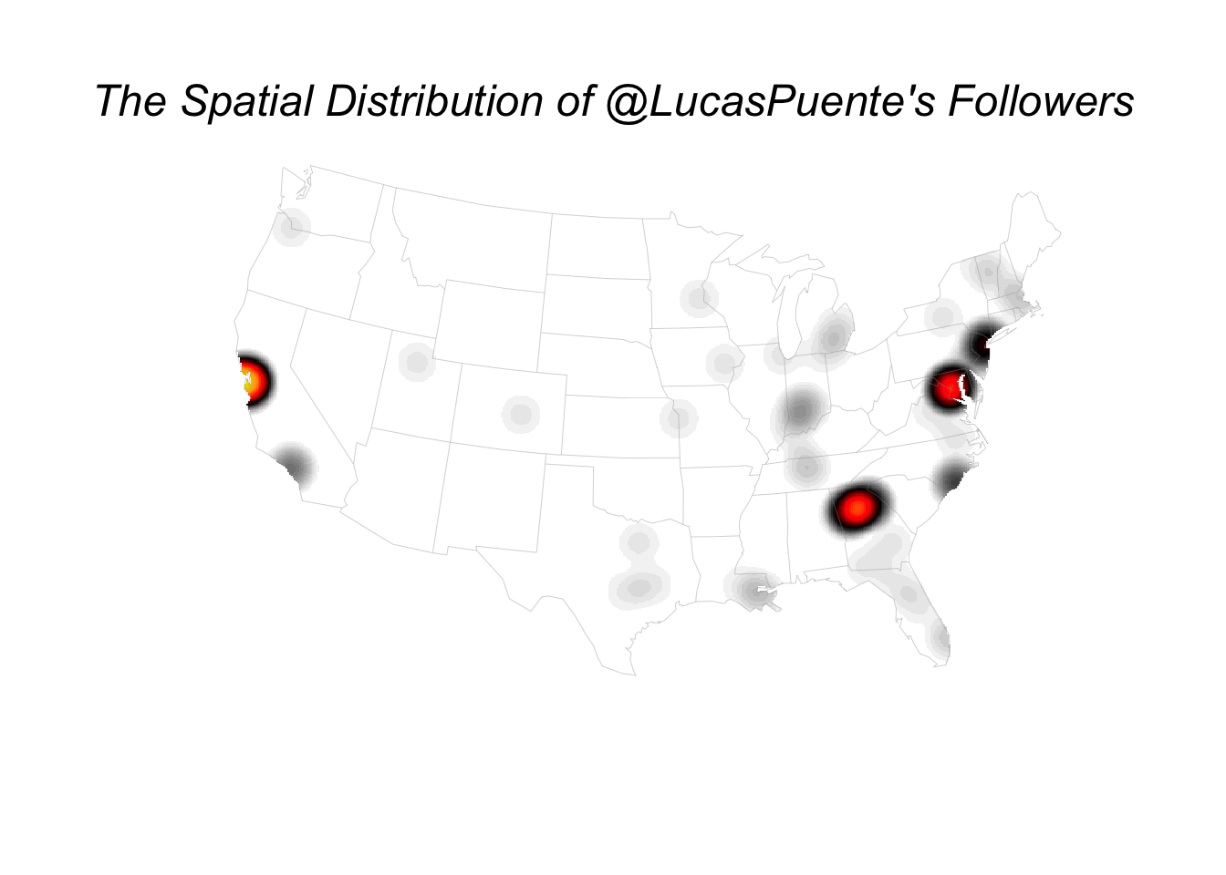
All of the code presented above is available in a single file on Github. If you have any other questions on how to map the locations of a user’s Twitter followers, please reach out, preferably via Twitter!


Site Design: jmcglone ![]()